Optimizing Search in Complex Networks

Chapter 1 Introduction

In this thesis, we investigate exploration and search on complex networks. Exploration on a network is the process of moving from site to site, based on a set of rules for moving, after starting at a site picked randomly or strategically, with the intention to cover sites. Searching, on the other hand, is the process of going from site to site, with the intention to find something hidden on some of those sites. There are many real-world scenarios involving search, e.g., a police officer searching for a thief hidden in some room in a hotel. Exploration or search is often carried out with a view to optimise it, or, in other words, make it time-efficient . In the earlier example of a police officer and a thief, the police officer would like to find the thief in the shortest time possible. And for that purpose, he would like to take the approach he deems the best for searching. This is where the concept of search strategy comes in. If there are several search strategies to pick from, then the search strategy that leads to the minimum time for searching, or, in other words, results in search optimisation, is called the optimal, or best performing, strategy. The process of searching is carried out by an entity (or multiple entities) that we call searcher. In the example of a police officer and a thief, the police officer is the searcher. The real-world scenarios involving a search for something, for the purpose of modelling them, can be formulated as a search game, where the searcher is carrying out search in the domain of search. In some of these scenarios, there is no hider in the picture that concealed objects, but there are just hidden objects. To model those scenarios, we assume there is a hider as well. And then those can be modelled as a game of hide-and-search, where the searcher is looking for the objects hidden by the hider, or, in some cases, looking to locate the hider only, in the domain of search. This thesis investigates search and exploration from a random walk perspective on complex networks. We study random walk search and exploration for families of degree- biased searching strategy. We take both analytical and numerical simulations route in this work and investigate the efficiency of the search and exploration measured by the number of items found and the number of distinct sites visited, respectively, per unit time during a random walk – for a variety of search strategies. That includes studies of the mean and the fluctuations of the search efficiency and its extreme value statistics. In what follows in this chapter, we will present a historical overview of the main topics relevant to this thesis, starting with random walks.

One of the most widely studied search strategies is a random walk. Random walks are processes comprising of a sequence of random steps on a graph, a continuous space, or a𝑛-dimensional lattice. The simplest example of random walks is a one-dimensional unbiased discrete random walk on a straight line where the walker can take a step of a uniform size backwards or forwards with equal probability. Random walks have been studied in relation to various fields, including physics, chemistry, computer science, and ecology over the years. Random walks are a class of stochastic processes. Some other stochastic processes [1] include the Brownian motion, Markov chains, diffusion, and the Wiener process. The connection between random walks and the other types of stochastic processes has been studied in detail over the years. Karlin and McGregor’s study of random walks as class of Markov chains [2] serves as an example. In one of the early advances in the field of random walks, Kac explored the resemblance between random walks and Brownian motion [3]. An overview of stochastic processes until the 1950s can be found in Doob’s article [4]. The problem of the random walk was first formulated by Pearson [5] in 1905, though it is thought to have first appeared before, as discussed by Carazza [6]. Random walks attracted some research interest over the next few decades [7]. The decade of the 1950s saw a remarkable increase in the research interest in random walks. Some studies on that front include the investigation of distribution and moments of passage times of random walks by Harris et al. [8], the study by Hodges el al. on moments of recurrence times of random walks [9], and the study of random walks with restrictions by Fisher et al. [10]. A history of random walks, including a variety of applications of random walks, is provided by Klafter et al. [11]. There have been many studies on random walks since the 1960s and random walks have found applications in a variety of fields. A survey [12] of the theory and applications of random walks on networks is provided by Masuda et al., where they confine their review to the cases of single and non-adaptive random walkers. Random walks have a wide range of applications, ranging from ecology [13] [14] to stock market [15] [16]. A review of random walks and their applications is provided by Klafter et al. [11]. Many types of random walks have been investigated over the years. The list includes L´evyﬂights [17], which are characterised by a heavy-tailed probability distribution for their step lengths, and which have real-world significance. As an example, L´evyﬂights have found applications in animal behaviour [18]. We also have in the list intermittent random walks [19], which are characterised by the rule that, at any step, the walker can go to one of its neighbours with probability𝛼, lying between 0 and 1, and jump oﬀthe domain of random walk with probability 1−𝛼. Another type of random walks are random walks with restart (RWR), during which, at any step, the walker makes a transition, with probability𝑟(0 𝑟 1), to one of its neighbours, or hops to the starting node (in case of a single starting node) with probability 1−𝑟. RWRs find application in image segmentation [20].

A popular type of random walk is the degree-biased random walk, where the walker is biased to go towards low or high degree nodes depending on the strategy. There are further categories of degree-biased random walks. In a major class of degree-biased random walk, at any time step, the probability of transition to a neighbour of degree𝑘is proportional to a function of𝑘. That function could be, for example, the square of𝑘, or the exponential of𝑘, out of infinitely many possibilities. Unbiased random walks can be seen as a special case of degree-biased random walks, with the bias is set to zero. Degree-biased random walks have attracted research interest of late [21] [22]. Degree-biased random walks are the random walk strategy we investigate in this thesis. Studies on random walks and their applications are in both discrete and continuous space. Some applications of discrete random walks are provided by Barber et al. [23]. Continuous-time random walks find applications in various fields, including chemotaxis [24], and finance and economics [25]. Studies of random walk search are not just limited to static networks. Perra et al., study random walk process [26] in time-varying networks in a regime where the connectivity pattern of the network and the dynamics of random walks are unwinding at the same time. Comparing their results with the past they demonstrate that the dynamic network connectivity pattern does have a significant impact on the search quality and dynamics. One of the prominent applications of random walks is in assigning relevance to results (in other words, documents) for a query on a click graph, as studied by Craswell et al. [27]. Search engines, such as Google, store each click on any search result displayed for a query as a query-document (or query-result) pair, and the count (the number of clicks) for a pair over a time period is an indicator, though weak indicator, of its relevance. Many truly relevant documents may not get clicked at all for a long time because they weren’t clicked in the first place. In their study, a random walk model is proposed and tested to probabilistically rank all documents such that those documents that are truly relevant but are without clicks get a more deserving ranking for a query. A study on adaptable search by Tsoumakos et al. stands out [28]. They test their search algorithm called adaptive probabilistic search method on peer-to-peer networks. Multiple walkers are set out for searching and the walkers are directed to sites based on the past search feedback, and in the process, sites (peers) make use of the topological information about their neighbours that they store. The authors demonstrate that their adaptive probabilistic search method is very eﬃcient, and there is quality learning from the feedback from past searches. In a study on local search strategies on power-law networks [29], Adamic et al. intro- duce a number of local random walk search strategies utilising the connectivity features of hubs and evaluate their performance. These random walk search strategies are tuned so that high degree nodes are visited more often than they would in case of an unbiased random walk. They also use the popular random walk strategies such as self-avoiding walks [30] and random walks with non-backtracking. They analyse the behaviour of search costs associated with searching as a function of the size of the network and demon- strate a sublinear scaling of search costs as a function of the network size. Their results show that, the scaling is better when their local search strategies biased towards high degree nodes are in use. There are many possible ways to evaluate the performance of a random walk search. Some of the prominent quantitative measures of random walks that have been studied over the years include the ﬁrst passage time (and the mean ﬁrst passage time) [31] [32], the cover time [33] [34], and the mixing rate [35] [36]. Search optimization is often a major goal of a search, including a random walk search. There have been many studies on optimising a random walk search [37] [38] [39]. In order to optimise a search, we need to the ﬁrst quantify the eﬃciency of the search, which can also be termed as the success rate of the search. One measure of the eﬃciency of a search is the ﬁrst passage time [40], which is the time step marked, by the ﬁrst arrival (of the walker) at a particular site on a network. If there is a hidden item in the picture then the target site for theﬁrst passage time could be the site concealing the item, and the source site could be picked at random. Or, the target site could be a site corresponding to the maximum degree in the network. There are multiple ways to select what two sites are the source and destination, respectively, for the ﬁrst passage time. If multiple random walks are being performed, then the resulting mean ﬁrst passage time [41] [31] can serve as a measure of the search eﬃciency. Going a step further from covering just one site, the time taken to cover a group of sites – which could be the sites containing the hidden items, in case of multiple hidden items – selected is a measure of the search eﬃciency. If multiple random searches are performed and the same number of items is hidden at nodes picked randomly, the search eﬃciency (based on this measure) might have a high variance across diﬀerent searches, even if those searches start from the same site in the network.

Another measure of the search eﬃciency is the time taken to cover all sites in the network, known as the cover time [42]. The cover time as a measure of the search eﬃciency is particularly of relevance to real-world problems where it is crucial to identify all hidden items, which could only be ensured by covering all the sites in the network. Cover time is a relatively robust measure of the search eﬃciency in the sense that the relative variance in the cover time is expected to be lesser than that for the ﬁrst passage time. Random walks have been an object of study as a search strategy in search games. Search games, introduced earlier in this chapter, are a category of games that involve searching in a search domain, also called search space. Among the many types of search games introduced and investigated over the years, there is the game of cops and robbers on graphs [43] [44], where mobile entities (cops) are attempting to track down another mobile entity (robber) on a graph. The rules are such that, at each time step, each cop can move to one of its neighbours, and following that, the robber can move to one of its neighbours, and this process repeats itself until the robber is found. Another type of search game investigated of late is the fugitive search game [45] [46], where the task is to trap a mobile fugitive hiding on a graph by placing searchers strategically. The fugitive has knowledge of the graph topology but can only move to vertices where cops are not present. Fugitive search games, along with the cops and robbers game are a type of pursuit-evasion games, which were introduced by Parsons [45]. There are many variants of these games. An overview of search games is presented by Garnev [47]. Search spaces for search games have a vast variety. Search games on Eulerian networks, trees and general networks are discussed and explored by Gal [48]. Search games on lattices have been a matter of study as well [49]. Search games go beyond discrete space. As an example, search games where the searcher can move along a continuous trajectory in their search for (mobile or immobile) hider were studied by Gal in 1979 [50]. Search games [48] have potential applications in a variety of the ﬁelds [47]. As an example, Fokkink et al. present applications of search games to counter terrorism studies [51]. Applications of search games in the ﬁeld of economics are discussed by Aumann et al. [52]. A recent comprehensive survey [53] of search games provided by Hohzaki covers many applications of search games. Hide-and-seek games involving a party searching for items hidden by another party are a class of search games. The term “hide-and-seek” is used in various contexts. As an example, Kikuta study a two-person zero-sum hide-and-seek game [54] where the network consists of a set of cells on a straight line, and the game requires the searcher to locate the hider hidden in one of the cells. There are travelling costs in the picture. Optimal strategies for the two players are found by Kikuta.

The hide-and-seek study mentioned in the above paragraph takes a game theory approach. In contrast, many studies take diﬀerent approaches. For an example, Chapman et al. take a random walk simulation approach to study hide-and-seek games, consisting of two players, a hider and a seeker [55]. The hider does the hiding on a network – with a bias towards a set of sites. The seeker carries out the search as per a random strategy and another strategy which is designed keeping the hiding bias in consideration. They show that depending on whether the hiding bias is uniform or not, the strategy with the hiding bias in consideration can perform better than the random strategy. We, in this thesis, study hide-and-seek games from a random walk simulation perspective where the hider conceals items randomly in a degree-biased fashion and the seeker performs degree-biased random walk search to locate the items. Games discussed so far have been studied on a variety of graph types and spaces as their domain. There have been many studies [56] [57] on a type of graphs called random graphs. An overview of random graphs is provided by Bollob´as [58]. A variety of synthetic random networks have been studied extensively over the years, and the main reason for that is their real-life signiﬁcance. The properties exhibited by these networks are found in many real-world networks, hence understanding a process on one of those networks gives us an idea of what it would be like in the corresponding real-world networks. These synthetic random network types include Erd˝os-R´enyi, scale-free and random regular, among others, and the three of them have been considered in this thesis, with Erd˝os-R´enyi being the most investigated one of the three. It was Erd˝os and R´enyi that ﬁrst studied properties of networks [59] where any two nodes have a link between them with probability𝑝, lying between 0 and 1, and not have a link with probability 1−𝑝. These networks were later called Erd˝os-R´enyi networks. The degree of distribution of these graphsﬁt a Poisson distribution. It was further observed that many real-world networks have a resemblance with Erd˝os-R´enyi graphs. There have been studies on the properties of Erd˝os-R´enyi graphs over the years [60], and rightfully so. Erd˝os-R´enyi graph is the main graph type studied in this thesis. Scale-free networks were ﬁrst introduced by Barabasi et al. [61]. Both directed and undirected scale-free networks have been a subject of investigation over the years [62] [63]. The occurrence of scale-free networks in real-world, from the rail network in China [64] to biological networks [65], has made them a topic of wide research interest. The degree distribution of scale-free networks resembles a power-law distribution. The long tail of the power-law degree distribution implies the presence of hubs – nodes with degrees much higher than the degrees of a majority of nodes. The presence of hubs makes scale-free graphs somewhat unique, and it, for instance, leads to a fast spread of information [66]. Studies by Barabasi et al. are some of the prominent and pioneering studies on scale-free graphs [67] [68] [63]. The studies on networks go beyond the networks discussed above. As an example, there have been studies on real-world peer-to-peer networks [69] [70]. In a study on power-law networks [29], Adamic et al. introduce some local random walk search strategies utilising the connectivity features of hubs and evaluate their performance. Perra et al. carry out studies on time-varying networks [26], especiﬁcally, they study the random walk process in time-varying networks in a regime where the connectivity pattern of the network and the dynamics of random walks are unwinding at the same time. In what follows next we refer to major tools used in our work and major works that inﬂuences our work.

A method that we use in our work, known as cavity approach, is often used in statistical physics to ﬁnd solutions to optimisation problems and was ﬁrst developed for spin glasses. The use of the cavity method goes beyond spin glasses [71], and covers, for instance, neural networks [72]. Martin et al. provide applications of the cavity method to optimisation problems in statistical mechanics [73]. It was in 2008 when, for the ﬁrst time, the cavity method was used to compute the spectra of sparse symmetric random matrices by Rogers et al. [74]. In the subsequent years the cavity method has been utilized for optimisation problems pertaining to, but not limited to, random matrices [75] [76]. Another concept that’s very relevant to our work is the concept of the thermodynamic limit, which refers to the limit of inﬁnite system size, and is an important concept in statistical physics. When dealing with systems (graphs, to be speciﬁc), it is sometimes desirable to ﬁnd very large system size behaviour. The magnitude of ﬁnite size eﬀects – the eﬀects due to the system size being ﬁnite – in systems (all systems encountered in real life have a ﬁnite size) can be large. Having an understanding of the ﬁnite-size eﬀects is important, and there have been studies on ﬁnite-size eﬀects [77]. Among many studies on thermodynamic limits, there is a work by Castellano et al. pertaining to scale-free networks [78] and a work related to spin glasses by Guerra et al. [79]. In this thesis, we also do computations in the thermodynamic limit using tools developed earlier. We use tools from Ku¨hn’s work on the spectra of sparse random matrices. In that work, a method to separate the contributions to the spectra of sparse random matrices coming from the giant cluster from those coming from the ﬁnite clusters is put forward. Ku¨hn made use of the methods, employed in Ku¨hn’s previous work [74] on computing the spectra for sparse matrices corresponding to the graphs belonging to the conﬁguration model class, and combined those methods with ideas developed around 2000 on studying percolation on random graphs. We use tools from that work, especiﬁcally, the tools for isolating the contribution from the giant cluster (given there is one) and the ﬁnite clusters from their work are the ones we use in this work. Analytical work of Chupeau et al., on cover times of random searches [33] is of relevance to our work. In their work, Chupeau et al. determine the distribution of cover times for a variety of random search strategies, including L´evy strategies [17], persistent random walks [80], random walks on complex networks [81] and intermittent strategies [82]. They demonstrate universal features of the distribution of cover times across various search strategies. They also study the optimisation of the mean cover time and illustrate that the search strategies optimizing the mean cover time also optimise the mean search time when just one item is hidden randomly on the network. They arrive at an analytical expression for the distribution of cover times and conﬁrm it with Monte Carlo simulations performed for the respective search strategies. We confirmed their result on the distribution of cover times𝜏for large𝜏. Now we brieﬂy describe our work. In our investigation of exploration and search using degree-biased random walk strategies, questions such as the following are addressed: What search strategy, or search parameter value maximises the eﬃciency of a search under given circumstances? How is the search eﬃciency, aﬀected by the graph topology, including the mean degree of the graph? What are eﬃcient hiding strategies for a given search strategy, from the hider’s perspective, and what are eﬃcient searching responses to a given hiding strategy, from the searcher’s perspective? What are some simple approximations to the search eﬃciency, which are good enough under speciﬁc conditions? Continuing from above, we also address the following questions: What is the nature of the ﬂuctuations in the exploration and search eﬃciency? How do theﬂuctuations in the exploration and search eﬃciency depend on the search strategy and features of the network? What conclusions can be drawn about the extreme value statistics of the network exploration eﬃciency? How best can a search strategy be improved during the search – based on the data from past search performance – in order to maximise the search performance, when repeated games are played?

In order to address these questions, we carry out numerical and analytical studies of random walk exploration and search on complex networks. We use existing methods to compute the average exploration eﬃciency and extend them to compute average search eﬃciency when hidden items are there in the picture as part of the hide-and-seek game on the network from a random walk perspective. Families of searching and hiding strategies are pitted against each other to ﬁnd searching responses that lead of search eﬃciency optimization under given hiding conditions and to ﬁnd eﬃcient hiding strategies for a given search strategy. We compute the exploration eﬃciency in the thermodynamic limit using available tools. We present simple approximations to search eﬃciency based on the ideas of equilibrium for the searcher and an eﬀective drift in random walks on networks, respectively. We study – through the numerical simulations route – the ﬂuctuations of the exploration and search eﬃciencies, and the distribution of maximum and minimum values of the exploration eﬃciency, taken over a set of independent random walk explorations. That includes the studies of the mean, variance, and quantiles of the exploration and search eﬃciency, and the dependence of those on the system size and the search strategy, in addition to studies of their probability distribution and the extreme value statistics of the network exploration eﬃciency. Next, with regard to real-time learning in an encounter and learning in repeated encounters, we try a variety of updates to the searching strategy based on the past hiding pattern and past success rate, so as to optimise the search. The quantiﬁcation of the search and exploration eﬃciencies in the hide-and-search dynamics in this thesis has been done diﬀerently to the three quantiﬁcations for random walks described earlier – the ﬁrst passage time, the cover time and the time taken to cover a subset of sites. This quantiﬁcation of the exploration and search eﬃciencies was carried forward from a work by De Bacco et al., [76]. We stick with the number of items found and the number of distinct sites visited per unit time as the measure of the search and exploration eﬃciencies, respectively. A part of our work is an adaptation of De Bacco et al.’s work on random walk exploration [76]. They investigated unbiased random walk exploration on complex networks. Their main result was that the number of distinct sites visited in theﬁrst𝑛time steps of an unbiased random walk is linear in𝑛, in the𝑛→ ∞limit, given 1≪n≪N, for 𝑁→ ∞. The coeﬃcient of linearity can be identiﬁed as exploration eﬃciency. They computed it using the cavity method. In this thesis, we investigate degree-biased random walks, as opposed to only unbiased random walks, and extend their results for that. We further have hidden items in the picture. We evaluate the search eﬃciency and study the hide-and-seek interplay for families of degree-biased hiding and searching strategies. As one of the prominent components of the thesis, we take a numerical simulations approach to study cover times on complex networks. This is largely in contrast to the approach taken by Chupeau et al., in their study of cover time [33], who mainly take an analytical approach. We confirmed a part of their result, which the cover time𝜏is exponentially distributed for large values of𝜏. In addition to the distribution of cover times, we study the behaviour of the mean cover time and its standard deviation as a function of the system size, and the change in mean cover time with a change in the mean degree of the network, all for Erd˝os-R´enyi graphs. And we experiment with a set of degree-biased random walk exploration strategies for our cover time study.

This remainder of this thesis is organised as follows. Chap. 2 describes the computa tion of the exploration and search eﬃciencies, our investigation of the interplay between random hiding and random walk searching strategies, and two approximations to the ex- ploration eﬃciency. In Chap. 3, we present a numerical analysis of ﬂuctuations of random walk exploration and search and the extreme value statistics of random walk exploration. Following that, in Chap. 4, we describe our investigation of learning for the seeker in the game of hide-and-seek, where the searching strategy can be adapted based on the past hiding information about the hider to improve the search performance. Finally, we summarise our work and brieﬂy discuss how our work can be carried forward in Chap. 5.

Chapter 3 Random Walk Exploration and Search on Complex Networks: Fluctuations and Extreme Values

Introduction

The idea of exploring a space or a network in a random fashion, formalised by the term random walk, has found relevance in many ﬁelds. There has been a signiﬁcant research interest on random walks on complex networks over the last many years [104] [105] [106] [107]. Random walks ﬁnd applications in a variety of ﬁelds, ranging from Biology [108] to economics [15]. A review of random walks and their applications is provided by Weiss et al. [109]. In this chapter, we carry out a numerical analysis of random walk exploration and search on complex networks. In particular, we investigate the ﬂuctuations of random walk exploration and search eﬃciencies, and the extreme value statistics of the random walk exploration eﬃciency. The analytical methods used in Chap. 2 to compute the average search and exploration eﬃciencies cannot compute quantities pertaining to the ﬂuctuations of random walks, for instance, the variance of the exploration eﬃciency. In this chapter, in order to study those quantities, we take a numerical simulation route. Fluctuations of random walks have attracted research attention in the past [110]. The ﬂuctuations are important to study since analysing the ﬂuctuations of a random walk related quantity can give the information about its distribution, mean, and percentiles, which, as stated earlier, have been investigated in this chapter. An extreme case of random walk exploration is when a random walk is performed until all the items are found, and the time taken for that is called the cover time. There have been studies on the cover time [111] [96]. Notably, there are two studies by U. Feige [112] [113] on the boundedness of the mean cover time, where the author provides upper and lower bounds as a function of the system size for random walks on graphs. These works served as a motivation for us to investigate the mean cover time as a function of the system size. An important work on cover times [33] by Chupeau et al., involves an analytical approach to study the cover times for a range of search strategies and graph types, including complex networks. They arrive at a universal analytical expression for the distribution of the cover times, which, for large𝜏, is nearly exponential in𝜏. They also carry out Monte Carlo simulations to complement their results. We conﬁrm their results for the distribution for large, through a numerical approach, as opposed to their largely analytical route. Our study ofﬂuctuations of random walk exploration and search and the extreme value statistics of random walk exploration is focused on two speciﬁc quantities resulting from random walks. The ﬁrst one is the number of distinct sites covered in the ﬁrst time steps of a random walk,𝑆(𝑛), and its search equivalent𝑆(𝜉,𝑛), which is the number of items found in the ﬁrst𝑛time steps of a random walk, and the two of them are measures of the exploration and search eﬃciency, respectively. The second quantity is the cover time, which is another measure of how good an exploration is.

In this chapter, there are four parts to our work. Firstly, we study the distribution of𝑆(𝜉,𝑛) and𝑆(𝑛), which helps us understand the nature of the ﬂuctuations of𝑆(𝑛) about 𝑆¯(𝑛). Next, we look at the distribution of extreme values (maxima or minima) of 𝑆(𝑛),taken over a set of𝑛-step random walks. It is followed by an investigation of the distribution of cover times and an examination of the behaviour of the mean cover time as a function of the mean degree and the system size. Finally, we look at extreme value statistics of cover times. We restrict ourselves to Erd˝os-R´enyi graphs in this chapter. Regarding random walk search (and exploration) strategies, we have mainly considered unbiased random walk search and degree-biased power-law random walk search. For hiding, we limit ourselves to purely random hiding and degree-biased hiding. The rest of the chapter is structured as follows. In Sec. 3.2, we discuss the past results on average search and exploration eﬃciencies and set a platform for the work described in this chapter. We present our investigation of the ﬂuctuations of exploration and search eﬃciency in Sec. 3.3.1. We discuss, in Sec. 3.3.2, the extreme value statistics of network exploration eﬃciency and discuss the Generalised Extreme Value distribution family. The Sec. 3.4 describes the theoretical aspects of our analysis of the cover time, including the ﬂuctuations and the extreme value statistics of the cover time. In Sec. 3.5, we present our results and the inferences derived, which is followed by the concluding remarks in Sec. 3.6.

Average Exploration Eﬃciency

In this section, we brieﬂy discuss the past results on the behaviour of 𝑆¯(𝑛). The quantity 𝑆¯(𝑛) is a measure of the average network exploration eﬃciency as discussed in chapter 2. Those results on the𝑛-dependence of 𝑆¯(𝑛) are described in Chap. 2 for degree-biased random walks, and also formulated in the work of De Bacco et al., [76] strictly for unbiased random walks. De Bacco et al. [76] formulated the following behaviour for 𝑆¯(𝑛) for unbiased random walk exploration (Eq. 2.4)

𝑆¯(𝑛) =𝐵𝑛 𝑓˜(︂ 𝐵𝑛 )︂ (3.1)

where the function 𝑓˜has the following asymptotic behaviour

𝑓˜(𝑦) ⎧1,𝑦≪1

⎩ 1 ,𝑦≫1

Another way to express the asymptotic behaviour (in the limit𝑛→ ∞) seen above in

3.1 and 3.2 is

𝑆¯(𝑛)∼𝐵𝑛,if𝜈≪1 (3.3)

𝑆¯(𝑛)≃𝑁,if𝜈≫1 (3.4)

In terms of𝜈≡𝑛/𝑁, with𝑁kept constant, and the quantity𝐵appearing in the equations above can be identiﬁed as the exploration eﬃciency. The quantity𝐵can be computed by using the cavity method, and also in the limit of inﬁnite system size, using an algorithm popularly known as the population dynamics, introduced by M´ezard and Parisi [102], as shown in chapter 2. In chapter 2, we showed that the Eqs. 3.3 and 3.4 hold for degree-biased random walk exploration too (Eq. 2.7), in addition to unbiased random walk exploration (Eq. 2.4). It can be shown that there is a functional dependence of 𝑆¯(𝑛) on𝑛and𝜈of the kind shown in Eqs. 3.1 and 3.2 for degree-biased searches too as well. For𝜈≪1 and𝑛≫1, there is a linearity in𝑛; for𝜈≫1, there is no dependence on𝑛; for intermediate𝜈, there is mostly a sub-linear dependence of 𝑆¯(𝑛) on𝑛, as highlighted in the previous chapter, and as discussed by De Bacco et. al., [76]. The main focus in chapter 2 was on the quantity 𝑆¯(𝑛), which, as discussed earlier, is the mean of𝑆(𝑛) – the number of distinct sites visited in𝑛time steps of a random walk search. In this chapter we go beyond the mean of𝑆(𝑛) and investigate the ﬂuctuations of𝑆(𝑛), using a numerical simulations approach. In particular, we study the distribution of𝑆(𝑛), including the variance and quantiles of the distribution too. In this chapter, in the numerical study of the two quantities – the cover time and 𝑆(𝑛) (and its search equivalent,𝑆(𝜉,𝑛)) – arising from random walks, a subset of random walk search strategies from Chap. 2 are used. Here, we mainly restrict ourselves to unbiased random walk exploration (Eq. 2.4) and search (Eq. 2.7), and power-law random walk search (table 2.1). We argue that our results with the above search strategies will qualitatively not be much diﬀerent from the results obtained when other search strategies are tried out. In the next section, we discuss the theory of the ﬂuctuations of𝑆(𝑛) about 𝑆¯(𝑛) and the extreme value statistics of𝑆(𝑛).

Exploration Eﬃciency

Understanding the probability distributions of𝑆(𝑛) and𝑆(𝜉,𝑛) is important from a real- world perspective. It could have applications in the real-world scenario where the task is to ﬁnd a number of treasures hidden in a set of sites selected from a vast network of sites. In the scenario it could be of interest to know how often a𝑛-step exploration or search is eﬃcient enough (the number of items found exceed a threshold value set for𝑆(𝜉,𝑛), or the number of distinct sites visited exceeds the a threshold value set for𝑆(𝑛)). We discuss the theory of the ﬂuctuations of𝑆(𝑛) in this section. In the example of treasures, it would be of interest to know how eﬃcient or ineﬃcient an exploration can be in extreme cases, which can be understood by studying the distribution of the maximum or minimum of𝑆(𝑛), taken over a set of random walks of length𝑛each. We later in this section discuss the extreme value statistics of𝑆(𝑛).

Fluctuations of Exploration Eﬃciency

We discuss the ﬂuctuations of the network exploration eﬃciency 𝑆(𝑛) in this part. We have already seen that𝑆(𝑛) is centered at 𝑆¯(𝑛)≡𝐵𝑛 𝑓˜(𝐵𝑛/𝑁), as given in Eq. 3.1. Equivalently, 𝑆¯(𝑛) is a function of𝜈and𝑛, and the limiting behaviours of 𝑆¯(𝑛) in𝑛is described in Eqs. 3.3 and 3.4. What could we say about the distribution of𝑆(𝑛) for 𝜈≪1? Is it symmetrical around 𝑆¯(𝑛)? We could ask such questions for𝜈=𝒪(1) or 𝜈≫1. Such questions can be addressed by studying the distribution of𝑆(𝑛). The distribution of 𝑆(𝑛) is qualitatively the same as the distribution of the number of items found in the ﬁrst𝑛steps, for the case when we have at maximum one hidden item per node, as we will later in Sec. 3.5. So understanding the distribution of𝑆(𝑛) gives us an understanding of the distribution of𝑆(𝜉,𝑛), and we restrict ourselves to𝑆(𝑛) in this section. We establish that the probability distribution𝒫(𝑆(𝑛)) of𝑆(𝑛) has the following scaling form

𝒫(𝑆(𝑛)) = 1 𝒫 (︂ 𝑆(𝑛)− 𝑆¯(𝑛) )︂ (3.5)

where𝜎(𝑛) is the standard deviation of𝑆(𝑛). The quantity𝑥(𝑛) appearing in the argument of the scaling function𝒫

𝑥(𝑛) = 𝑆(𝑛)−𝑆¯(𝑛)

represents a normalized deviation of𝑆(𝑛) from its mean. The scaling function𝒫(𝑥(𝑛)) is simply the probability density function𝑓(𝑥(𝑛)) of𝑥(𝑛). Weﬁnd that, the probability density function𝑓(𝑥(𝑛)) of𝑥(𝑛) is independent of𝑛and 𝑁, for 𝑛≫1, as we will see in Sec. 3.5. It does depend on the graph type and the random walk exploration strategy used. It is to be noted that we do not have𝑛≪𝑁as one of the requirements for the independence of the distribution of𝑥(𝑛) from𝑁and𝑛, which was a necessary condition for the linearity of 𝑆¯(𝑛) in𝑛. Once 𝑆¯(𝑛) and𝜎(𝑛) are known percentiles of the𝑆(𝑛) distribution are easily expressed in terms of percentiles of the (𝑛-independent) distribution of𝑥(𝑛). Regarding 𝑆¯(𝑛), its dependence on𝑛is already known (Eq. 3.1), and is described in section 3.2 for all𝜈, including𝜈in the limits𝜈≫1 and𝜈≪1. For the standard deviation𝜎(𝑛), from the numerical analysis, we ﬁnd that

𝜎(𝑛)∝𝑛 ^𝛾 (3.7)

Where, the power-law exponent ^𝛾= 0.4981±0.0012. Since the degree-biased random walks under consideration, particularly on large networks, have an eﬀective drift, these random walks resembles one-dimensional random walks with a drift, for which, it is known that 1 the standard deviation over a𝑛-step walk is proportional to𝑛 2 . Given the resemblance, the true power-law exponent in our case may be 1/2. Now we shift our focus to the cumulative distribution of𝑥(𝑛) and the percentiles of 𝑆(𝑛). Given that the distribution of𝑥(𝑛) does not depend on𝑛and𝑁, as long we have 𝑛≫1, we will henceforth mostly refer to𝑥(𝑛) as𝑥. In terms of the probability density function𝑓(𝑥) of𝑥, the cumulative distribution𝐹(𝑥) of𝑥can be written as

𝐹(𝑥) =𝑓(𝑥)d𝑥 (3.8)

For a pair of values of𝑛and𝑁, and a given𝑥 *, we have

𝐹(𝑥 *) =𝑃(𝑥≤𝑥 *)

=𝑃 [︂ 𝑆(𝑛)− 𝑆¯(𝑛) ≤ 𝑆* − 𝑆¯(𝑛) ]︂

=𝑃(𝑆(𝑛)≤𝑆 *) (3.9)

where𝑆 * is the value of𝑆(𝑛) that satisﬁes 𝑆 * = 𝑆¯(𝑛)+𝑥*𝜎(𝑛). We see that the probability distribution of𝑆(𝑛) can be written in terms of the cumulative distribution of𝑥. From the cumulative distribution of𝑥, we know the𝑝’ percentile𝑥 𝑝 of𝑥. In terms of𝑥 𝑝, we then have

𝑆𝑝 = 𝑆¯(𝑛) +𝑥 𝑝𝜎(𝑛) (3.10)

as the𝑝’th percentile of𝑆(𝑛). Now that we can compute percentiles of𝑆(𝑛), we fully know its distribution, which could have real-life implications, as we will see in Sec. 3.5. In the following section, we look at the extreme values (maximum and minimum) of𝑆(𝑛), taken over a set of independent random walks.

Extreme Values of Exploration Eﬃciency

As an application of the extreme value statistics of𝑆(𝑛), we can think of the earlier example of treasures. It would of interest to know how eﬃcient or ineﬃcient a search or exploration can be at its extremes over multiple random walk searches of𝑛-step each. In this section, the focus is on the extreme values of𝑆(𝑛) over a set of independent random walks of length𝑛each. We show how the distributions of maximum and minimum of𝑆(𝑛) are related to𝐹(𝑥) (Eq. 3.9). Later, we outline the existing results in extreme value theory and discuss them in relation to the quantities of interest in our study.

3.3.2.1 Extreme Values: Formulation and Distribution

In this part we show how the distributions of maximum and minimum of𝑆(𝑛) are related to𝐹(𝑥) (Eq. 3.9). We deﬁne,

𝑀𝑠(𝑛) = max 𝑆𝑟(𝑛) (3.11)

as the maximum number of distinct nodes covered over𝑠independent random walks of length𝑛each, where𝑆 𝑟(𝑛) is the number of distinct nodes covered in theﬁrst𝑛time steps of the𝑟’th random walk. The quantity𝑆 𝑟(𝑛) is not to be confused with the quantity 𝑆𝑖(𝑛) used in Chap. 2, which was a convenient way of expressing 𝑆¯𝑖(𝑛), which referred to the average number of distinct sites visited over multiple𝑛-step random walks started at node𝑖. Similar to𝑀 𝑠(𝑛), we deﬁne,

𝑚𝑠(𝑛) = min 𝑆𝑟(𝑛) (3.12)

as the minimum number of distinct nodes covered over𝑠independent random walks of length𝑛each. We further have 𝑀¯ 𝑠(𝑛) as the averaged maximum number of distinct visited in𝑛time steps, averaged over a large number of sets of𝑠independent random walk explorations of length𝑛each. Similarly, we have ¯𝑚𝑠(𝑛) as the averaged minimum number of distinct sites visited in the ﬁrst 𝑛time steps. We will see later in Sec. 3.5 the behaviours of𝑀 𝑠(𝑛), 𝑀¯ 𝑠(𝑛), and ¯𝑚𝑠(𝑛) as functions of𝑠. Now we turn to formulating the cumulative distributions of the extreme values𝑀 𝑠(𝑛) and𝑚 𝑠(𝑛). For the sake of completeness, we outline how the distribution of extreme values of𝑆(𝑛) can be written in terms of the cumulative distribution of𝑆(𝑛), or, equivalently, the distribution of the normalised deviation𝑥(𝑛) of𝑆(𝑛). The probability that𝑀 𝑠(𝑛) takes a value less than𝑆(𝑛) =𝑆 * can be written as

𝑃(𝑀 𝑠(𝑛)≤𝑆 *) =𝑃[(𝑆 1(𝑛)≤𝑆 *)∩(𝑆 2(𝑛)≤𝑆 *)∩....∩(𝑆 𝑠(𝑛)≤𝑆 *)]

=𝑃(𝑆 1(𝑛)≤𝑆 *)×𝑃(𝑆 2(𝑛)≤𝑆 *)×....×𝑃(𝑆 𝑠(𝑛)≤𝑆 *)(3.13)

where we have used the theorem that the probability of the intersection of a set of independent events is the product of individual probabilities. Further, using Eq. 3.9, the Eq.

3.13 results in

𝑃(𝑀 𝑠(𝑛)≤𝑆 *) = [𝐹(𝑥 *)]𝑠 (3.14)

where𝑥 * has the same deﬁnition as given in Sec. 3.3.1 – it satisﬁes 𝑆 * =𝑥 *𝜎(𝑛) + 𝑆¯(𝑛). Thus the cumulative distribution of𝑀 𝑠(𝑛) can be written in terms of𝐹(𝑥). Also, we can

compute percentiles of𝑀 𝑠(𝑛) in terms of percentiles of𝑥.

Similarly, for𝑚 𝑠(𝑛), we have

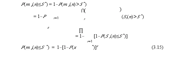
Where, we have used one of the fundamental rules of probability, in addition to Eq. 3.9. As given in Eq. 3.15, the cumulative distribution of𝑚 𝑠(𝑛) can be written in terms of 𝐹(𝑥). We could also write percentiles of𝑚 𝑠(𝑛) in terms of percentiles of𝑥(𝑛), or even percentiles of𝑆(𝑛), as percentiles of𝑆(𝑛) and percentiles of𝑥(𝑛) are related to each other (Eq. 3.10). Now we look at some existing results for extreme value statistics, especiﬁcally, the Generalised Extreme Value (GEV) theory and distributions.

3.3.2.2 Generalised Extreme Value Distributions

As per the Generalised Extreme Value (GEV) theory for a random variable, the probability distribution of its extreme values can fall into one of the three families of dis tributions [114] given by the theory, which are known as GEV distributions. When the values the random variable can take are bounded, the theory states the distribution of the random variable belongs to the Weibull family, deﬁned by Eq. 3.17. For random variable 𝑆(𝑛), we ﬁnd by data ﬁtting that the distribution of its maximum𝑀 𝑠(𝑛) obtained from stochastic random walk simulations belongs to the Weibull family, as one would expect, given that𝑆(𝑛) is bounded from below and above. As per those results, it is evident that the Weibull cumulative distribution of𝑀(writing𝑀 𝑠(𝑛) as𝑀forﬁxed𝑛and𝑠) is

The expected values of the variable𝑀and its variance, respectively, are

𝐸(𝑀) =𝜇− 𝜉˜ − 𝜉˜𝑔1 (3.18)

with𝑔 𝑘 =Γ (︁1−𝑘 𝜉˜)︁ ,whereΓ(.) is the standard Gamma function.

Regarding the minimum𝑚 𝑠(𝑛) of𝑆(𝑛), it can be seen that𝑚 𝑠(𝑛) (≡min 𝑟=1,...,𝑠 𝑆𝑟(𝑛)) is equivalent to “𝑛−max 𝑟=1,...,𝑠 (𝑛−𝑆 𝑟(𝑛)),” which is bounded above by𝑛and bounded below by zero. The probability distribution of𝑚 𝑠(𝑛) is Weibull, and its cumulative probability distribution has the same structure as given in Eq. 3.16. Now we switch to cover times.

Cover Time Analysis

The cover time is a useful quantity from a real-world perspective. As an application of cover times, we can think of the following. Suppose the elements of a sensitive information, so sensitive that it is very important to ﬁnd those elements, are hidden in a couple of sites in a big connected network. Or, suppose a bomb is hidden at a couple of sites taken from a large connected network. Then we would like to make sure every single one of them is found. And to have an idea of how long it might take on an average to ﬁnd all of them, we can study the mean of the cover time, and more generally, the distribution of the cover time. The analytical distribution of cover times on Erd˝os-R´enyi graphs was given by Chu- peau et al. [33]. Our study of the distribution of cover times is done from a numerical point of view, as opposed to the primarily analytical study of cover times by Chupeau et al., where they present a universal expression for the distribution of cover times valid for many random walk types. We conﬁrm one of their results that the shape of the distribution of cover times𝜏for large𝜏is exponential in𝜏. In this section, we present the theoretical concepts regarding our numerical study of cover times, which involves an investigation of multiple aspects of cover times obtained from stochastic random walk simulations on complex networks. Our study on cover times only concerns Erd˝os-R´enyi graphs. We study the distribution of cover times. We analyse the behaviour of the mean cover time – the average value of the cover time taken over many random walks – as a function of the mean degree, and also as a function of the system size. We also examine the statistics of the extreme values of cover times, taken over a set of independent random walks.

Distribution of Cover Times

In this part, we ﬁrst discuss the distribution of cover times𝜏and the ﬂuctuations in𝜏 about its mean⟨𝜏⟩. From the distribution of cover times𝜏observed, it is noted that the distribution is very much diﬀerent for small and large values of𝜏. For large𝜏(speciﬁ- cally, 𝜏>𝜏 0, for a threshold value𝜏 0), it turns out the probability density𝑃(𝜏) decays exponentially in𝜏:

𝑃(𝜏)∝𝑎 −𝑏𝜏 (3.20)

Where, 𝑎and𝑏 are positive constants. This is an already established result of Chupeau et al. [33]. More generally, they present an analytical expression for𝑃(𝜏) for all𝜏. The values of constants𝑎and𝑏can be obtained by proper data ﬁtting. We see that𝑏>1. The mean and variance are often the most studied features for a probability distri bution. We look at these two features of the distribution of cover times as a function of the system size. The mean cover time⟨𝜏⟩ 𝑁 (⟨𝜏⟩for a system of size𝑁) is found to be a power-law function of the system size –⟨𝜏⟩ 𝑁 follows

⟨𝜏⟩ 𝑁 ∝𝑁 (3.21)

for power-law exponent𝛾. For the search strategies tried so far, we ﬁnd𝛾>1. We also observe that, a better search strategy as per our measure of the search performance (one that leads to a larger𝐵) generally results in a larger𝛾.

For the standard deviation𝜎 𝜏 (𝑁) (on graphs of size𝑁) of𝜏, we ﬁnd the following relation

𝜎𝜏 (𝑁)∝𝑁 𝜒 (3.22)

where the power-law coeﬃcient𝜒>1 . For various search strategies tried out on Erd˝os- R´enyi graphs, we ﬁnd that𝜒 𝛾.

Normalised Fluctuations and Extreme Values

Now we turn to the distribution of the ﬂuctuations of the cover time and the extreme value statistics of the cover time. We start by deﬁning the normalised ﬂuctuation of𝜏as

𝑧(𝑁) = 𝜏(𝑁)− ⟨𝜏⟩ /𝜎𝜏 (𝑁)

For a given𝑁and𝑧=𝑧 *, we have the following expression for the cumulative distribution 𝐹(𝑧) of normalised deviations𝑧(𝑁)

𝐹˜(𝑧 *) =𝑃(𝑧 𝑧 *)

=𝑃 [︂ 𝜏(𝑁)− ⟨𝜏⟩ ≤ 𝜏 * − ⟨𝜏⟩ ]︂

=𝑃(𝜏(𝑁)≤𝜏 *) (3.24)

where𝜏 * is the value𝜏(𝑁) takes that satisﬁes 𝜏 * =𝑧 *𝜎𝜏 (𝑁) +⟨𝜏⟩. We see that the distribution of the normalised ﬂuctuations of𝑧(𝑁) is related to the distribution of𝜏(𝑁) in the same manner as the distribution of normalised ﬂuctuations of𝑆(𝑛) is related to the distribution of𝑆(𝑛), as outlined towards the end of Sec. 3.3.2.1. From the cumulative distribution of𝑧, we know the𝑝’th percentile𝑧 𝑝 of𝑧. In terms of𝑧 𝑝, we then have

𝜏𝑝 =⟨𝜏⟩+𝜎 𝜏 (𝑁)𝑧 𝑝 (3.25)

as the𝑝’th percentile of𝜏(𝑁).

Now coming to the extreme value statistics of cover times, the theory of the statistics of extreme (maximum or minimum) values of the cover time taken over a set of random walks is identical to the theory of the statistics of extreme values of𝑆(𝑛). That includes expressing the cumulative probability distribution of extreme values in terms of the probability distribution of ﬂuctuations of extremes values, as done in Sec. 3.3.2.1, and Weibull distribution ﬁt of the distribution of extreme values of cover times, as done in section

3.5 Results

In this section, we present our results for numerical studies of random walk exploration and search. We also touch upon potential real-life applications. To begin with, we show our ﬁndings on the ﬂuctuations of𝑆(𝑛). Then we move to the extreme value statistics of𝑆(𝑛). Finally, we discuss the results obtained for cover times – including the ﬂuctua- tions/distribution of𝜏, the behaviour of mean cover time⟨𝜏⟩as a function of𝑐and𝑁, and the extreme value statistics of𝜏(𝑁). In the present chapter, we largely investigate network exploration, where the objective is not to ﬁnd any items that may be hidden but it is to cover sites of the network. The distribution of the normalised ﬂuctuations of𝑆(𝑛) for network exploration is similar to the distribution of the normalised ﬂuctuations of𝑆(𝜉,𝑛) – the number of items found in 𝑛time steps of a random walk – as long as other factors, such as the search strategy, are kept unchanged. So network exploration (no items hidden) captures the qualitative behaviour one would see for hiding (table 2.1) too. In this chapter, in addition to unbiased exploration and search, we also investigate power-law search (table 2.1). We will show later in this section that the shape of the normalised probability distribution of𝑆(𝑛) does not change much with changing the search strategy, as long as𝑛≫1. [[It may also hold for the distribution of extreme values of𝑆(𝑛) – taken over a set of random walks – and the distributions ofﬂuctuations and extreme values of cover times. ]] In conclusion, at least for theﬂuctuations of𝑆(𝑛), carrying out just unbiased search suﬃces in order to know the qualitative nature of its probability distribution. In this section, unless stated otherwise it can be assumed that the network under consideration is an Erd˝os-R´enyi network. Regarding search strategies, the default search strategy considered in this chapter for both search and exploration is an unbiased random. Next, we show our results on theﬂuctuations of𝑆(𝑛).

3.5.1 Fluctuations of Network Exploration and Search Eﬃcien- cies

Figure 3.1: Normalised distribution (the blue curve) of𝑆(𝑛) for𝑛= 400 when degree- biased power-law random walk exploration (with𝛼= 1) is done. Shown is result on Erdos-Renyi graph with𝑐=4 and𝑁=6000. Highlighted are the 1st (green line), the 99th (red line) percentile and the mean (black line). The 1st percentile is 250, the 99th percentile is 302, and the mean value is 276.7466.

The normalised distribution of𝑆(𝑛) for a degree-biased power-law random walk exploration is shown in Fig. 3.1. A close look at the ﬁgure reveals that the normalised

Figure 3.2: Normalised distribution of𝑆(𝑛)/𝑛for diﬀerent pairs of values of𝑛and𝑁, when𝑛/𝑁is kept constant. Unbiased random walk exploration performed on Erd˝os- R´enyi graph with mean degree four. The curves in the central region from bottom to top correspond to increasing𝑛.

Distribution is not symmetrical about the mean (the black line), not about any line for that matter. The degree of asymmetry is quite dependent on the search parameter𝛼. Asymmetry increases when𝛼is switched to 1 from 0, for instance. As an application of this, one could think of the real-world scenario mentioned earlier where a number of treasures are hidden in some fashion in a group of sites selected from a vast network of connected sites. One might be interested in knowing how many sites are likely to be covered in a speciﬁed number of steps with a 99 % chance. To address questions like that, we have shown the 1st and the 99th percentile in the ﬁgure. In this particular case, as 302 is the 99th percentile, one would discover 302 sites in a walk of 400 steps 99 out of 100 times on an average.

The distribution of𝑆(𝑛) is centered at

𝑆¯(𝑛), and, equivalently, the distribution of 𝑆(𝑛)/𝑛is centered at 𝑆¯(𝑛)/𝑛, but one might wonder what we could say about the variance of the distribution of 𝑆¯(𝑛)/𝑛, or whether the distribution is symmetric around 𝑆¯(𝑛)/𝑛. In Fig. 3.2, we see the normalised distribution of𝑆(𝑛)/𝑛for four diﬀerent pairs of values of 𝑛and𝑁, keeping𝑛/𝑁the same, for unbiased random walk exploration on Erd˝os-R´enyi graphs of mean degree four. As one can see the curves are not symmetrical about any line. Further, the four curves do not peak at the same value of𝑆(𝑛)/𝑛.

Fig. 3.3 displays the distribution (left panel) of the normalised deviation𝑥(𝑛), formulated in Eq. 3.6, for multiple pairs of values of𝑛and𝑁. We can express𝑥(𝑛) as𝑥 𝑁 (𝑛) for variable𝑁, as is the case here. Here all the curves correspond to just one graph type – Erd˝os-R´enyi – and the mean degree of four. Across the four curves shown pairs of values of𝑛and𝑁picked are such that: there are diﬀerent value of𝑛for the same𝑁, there are

Figure 3.3: Normalised distribution of𝑥is shown in both the plots. The values𝑥 𝑁 (𝑛) obtained from random walk explorations on Erd˝os-R´enyi graph with𝑐=4. Left panel: distribution of𝑥 𝑁 (𝑛) for diﬀerent pairs of values of𝑛and𝑁. It can be seen that the distribution of𝑥 𝑁 (𝑛) is universal in the range of small𝜈(=𝑛/𝑁) as long as the graph type, the mean degree and the search strategy are kept unchanged. In the right panel, normalised distribution of𝑥 𝑁 (𝑛) for diﬀerent values of𝜈, for a given𝑁. It can be seen that the distribution of𝑥 𝑁 (𝑛) is same for all𝜈that ensure𝑛 1, as long as the graph type, the mean degree and the search strategy are kept unchanged.

Figure 3.4: Normalised distribution of𝑥for diﬀerent values of the search parameter𝛼for the power-law exploration. Erd˝os-R´enyi graphs of size 4800 and mean degree four considered. Exploration performed for𝑛= 400 steps. As one could see the qualitative behaviour does not change with changing𝛼, so one could use any value of𝛼(including𝛼= 0 – unbiased exploration/search) to know the qualitative behaviour, and we mostly stick with unbiased search/exploration.

Figure 3.5: In the left panel, we see the change in𝜎(𝑛) (resulting from unbiased random walks) with respect to𝑛on Erd˝os-R´enyi graphs of size 6400 and mean degree four. In the right panel we see the corresponding double logarithmic plot. The straight-line nature of the plot implies that𝜎(𝑛) has a power-law dependence on𝑛. The power-law exponent is found to 0.4981±0.0012.

diﬀerent values of𝑁for the same𝑛, there are same values of𝑛/𝑁, and there are diﬀerent values of𝑛/𝑁. But there is one thing common across the four pairs of values of𝑛and𝑁 they all result in the same normalised distribution of𝑥 𝑁 (𝑛). The overlap of normalised distributions is conditional on having the same graph type, the same mean degree and the same search strategy, and also the condition𝑛≫1, as we will see later. Fig. 3.3 shows the distribution of𝑥(𝜈) (Eq. 3.6, with𝑛=𝜈𝑁, and constant𝑁) for various values of𝜈(right panel). Again, all the curves correspond to just one graph type Erd˝os-R´enyi – and the mean degree of four. Across the four curves shown a range of values of𝜈have been tried out, keeping𝑁constant. It can be seen that the normalised distributions of𝑥(𝜈) fall on top of each other for all values of𝜈considered other than 𝜈= 1/64, which amounts to𝑛= 100. Our understanding is that it is because of the fact that the criterion𝑛≫1 is not met for that value of𝜈. It shows we can expect the same distribution for diﬀerent values of𝜈, as long as𝑛≫1, and we have the same graph type, the same mean degree and the same search strategy. As seen in Fig. 3.3 (both left and right panel), the distribution of𝑥 𝑁 (𝑛) is independent of𝑛and𝑁, as long as𝑛≫1 and𝑁is large. From the cumulative probability distribution 𝐹(𝑥) of𝑥, we know the𝑝’th percentile𝑥 𝑝 of𝑥for any𝑝. Consider the real-world example mentioned earlier where a party is trying to ﬁnd a set of treasures hidden in a vast network of sites, maximum one at each site, and is looking to encounter as many new sites as possible during the search. It might be of interest to know how many distinct sites a random walker visits, in an average sense, 95 percent of the time, in a random walk of length 200. The desired number is𝑆 95 = 𝑆¯(200) +𝜎(𝑛)𝑥 95, as obtained from Eq. 3.10.

Figure 3.6: Extreme values of𝑆(𝑛) (left panel) and their average (right panel) as a function of𝑠when unbiased exploration of 200 time steps is performed on Erdos-Renyi graph of𝑁=6000 nodes and𝑐=4. Left panel: the evolution of𝑀 𝑠(𝑛) as a function of 𝑠for a particular (growing) sequence of random walks. Right panel: Both 𝑀¯ 𝑠(𝑛) (blue curve) and ¯𝑚𝑠(𝑛) (red curve) as a function of𝑠, averaged over 10000 sets of sequences of 𝑠random walks.

We study the standard deviation𝜎(𝑛) of the probability distribution of𝑆(𝑛) for various values of𝑛(keeping the graph type,𝑁,𝑐and the search strategy unchanged). Fig. 3.5 shows the behaviour of𝜎(𝑛) as function of𝑛(left panel). The right panel shows the result on a double-logarithmic plot, and the straight-line behaviour obtained translates to power-law dependence in the standard/linear scales. Thus, we ﬁnd that the standard deviation𝜎(𝑛) has a power-law dependence (Eq. 3.7) on𝑛. The power-law exponent ˜𝛾for the power-law dependence comes out to be 0.4981 ±0.0012, a value close to 1/2. The degree-biased random walks under consideration, particularly on large networks, have an eﬀective drift, these random walks resembles one- dimensional random walks with a drift, for which, it is known that the standard deviation 1 over a n-step walk is proportional to𝑛 2 . Given the resemblance, the true power-law exponent in our case may be 1/2. In Fig. 3.4, the distribution of normalised ﬂuctuations𝑥(𝑛) is shown for multiple values of the search parameter𝛼for power-law exploration, which is performed on Erd˝os- R´enyi graphs of size 4800 and mean degree four. The shape of the distribution does not change much with changing𝛼, so we could stick with a random value of𝛼to get an idea of the behaviour expected for any value of𝛼. We mostly stick with𝛼= 0, which amounts to an unbiased random walk. In the next part, we present our results for the extreme value statistics of𝑆(𝑛).

3.5.2 Extreme Value Statistics of Network Exploration Eﬃciency

Figure 3.7: Normalised distribution of𝑀 𝑠(𝑛) observed from the data obtained from simulations (sim. in the plot) and the Weibull distributionﬁt, for two diﬀerent values of𝑠. Unbiased network exploration of𝑛=400 steps done on Erd˝os-R´enyi graph of 6400 nodes and mean degree 4. Goodﬁt is observed in most areas.

With regard to our study of the extreme value statistics of𝑆(𝑛), ﬁrst we look at the behaviour of𝑀 𝑠(𝑛) (left panel) as a function of𝑠– the number of random walk walks over which the maximum is taken, for𝑛= 200, for a sequence of random walks, which is shown in Fig. 3.6. There are only a few values of𝑠in the given range where we see a jump in𝑀 𝑠(𝑛). Each of those values corresponds to a random walk instance in which the number of distinct sites visited is more than the number of distinct sites visited in any random walk instance before. In the right panel of Fig. 3.6 we see the behaviour of 𝑀¯ 𝑠(𝑛) – the average of𝑀 𝑠(𝑛) over a large number of sets of𝑠random walk realisations each – for𝑛= 200, as a function of𝑠. As expected, 𝑀¯ 𝑠(𝑛) is an increasing function of𝑠. Investigating the distribution of 𝑀¯ 𝑠(𝑛) from the logarithmic plot (right panel) dis played in Fig. 3.6, it is revealed that there is a regime of𝑠in which the𝑠-dependence of𝑀 𝑠(𝑛) is power-law in nature, 𝑀¯𝑠 ∼𝑠 ^𝑎. The power-law exponent ^𝑎is 0.026±0.0003. The quantity ¯𝑚𝑠(𝑛) can also be seen in the same ﬁgure. For ¯𝑚𝑠, we ﬁnd the power-law exponent ^𝑏for the weak power-law behaviour ( ¯𝑚 ∼𝑠 ^𝑏) to be−0.032±0.0005. For small Values of𝑠, the dependence of 𝑀¯ 𝑠(𝑛) on𝑠is weaker than any power-law. It is to be noted That the rate of change of 𝑀¯ 𝑠(𝑛) with respect to𝑠is decreasing as𝑠is increasing, which is something one would expect. It is of interest to know how many treasures at maximum or minimum can one ﬁnd with a 90 percent chance, in random walks of 1000 steps, as it could have potential applications, including in the real-world scenario mentioned earlier where a person is trying to ﬁnd a number of treasures hidden in a random set of sites taken from a vast network of sites.

Figure 3.8: Left panel: Change in the parameter𝜇for Weibull distributionﬁt (appearing in Eq. 3.16) with respect to a change in the parameter𝑠. Erd˝os-R´enyi graph of𝑁=6000 nodes and𝑐=4 considered. Unbiased network exploration performed. In the right panel, we see both axes in the log scales. The dependence of𝜇(𝑠) on𝑠is weaker than a power-law.

Such questions can be addressed by knowing the cumulative probability distribution of 𝑀𝑠(𝑛) (to be precise, we need to know the probability distribution of the maximum of the number of items found over𝑠random walks of𝑛steps each, but as argued before, its distribution is expected to be similar to the distribution of𝑀 𝑠(𝑛)). The cumulative probability distribution of𝑀 𝑠(𝑛), is shown in Fig. 3.7 for a case of unbiased random walks. The distribution of𝑀 𝑠(𝑛) (written as𝑀, for a given𝑠and𝑛, as given in Eq. 3.16) for two diﬀerent values of𝑠is shown in Fig. 3.7. For each value of𝑠, the parameters𝜇,𝜎and 𝜉˜(Eq. 3.16) are obtained by ﬁtting the data of extreme values (maximum, in the present case). Weﬁnd it is the Weibull class of the Generalised Extreme Value distributions that the data falls into, as conﬁrmed by the negative sign of the shape parameter 𝜉˜. We can see that theﬁt to the Weibull distribution is not as good around the value of𝑛corresponding to the peak, for the two values of𝑠considered. We do observe that the ﬁt, at least around the peak, gets better as𝑠is increased from 100 to 200. As per the theory, theﬁt would be perfect for𝑠→ ∞. The ﬁt is expected to get better with an increase of𝑠, which is what we observe too. The distribution of𝑚 𝑠(𝑛) is also found to belong to the Weibull extreme value class. In Fig. 3.8 we see the𝑠-dependence of one of the ﬁtting parameters of Weibull distribution. Speciﬁcally, we see the change in the parameter𝜇with a change in parameter𝑠. The dependence of𝜇on𝑠is sub power-law. In the next part, we discuss our results on cover times.

3.5.3 Cover Time Analysis

We investigate cover times obtained through random walk simulations. The distribution of cover times obtained when unbiased random walk exploration is performed on Erd˝os- R´enyi graphs of mean degree four, is shown in Fig. 3.9. The red line parallel to the vertical axis (left panel) represents the mean cover time⟨𝜏⟩. For large𝜏, or𝜏>⟨𝜏⟩, it is helpful to have the probability density in the logarithmic scale in order to better see the distribution, as done in the right panel. As we increase𝜏in the range of large𝜏, we observe that𝑃(𝜏) decays exponentially after a certain threshold value𝜏 * of𝜏, which, in this particular case, is not too far from⟨𝜏⟩. It can also be said from the ﬁgure that, the peak of the probability distribution doesn’t have to correspond to the mean value of the cover time. The observation that the probability distribution of𝜏is exponential in nature for large 𝜏, is a conﬁrmation of one of the ﬁndings of Chupeau et al. [33] on complex networks. In an analytical work on cover times of random searches [33], Chupeau et al. determine the distribution of cover times for a variety of random search strategies, including random walks on complex networks [81] and intermittent strategies [82]. They demonstrate universal features of the distribution of cover times across various search strategies. They arrive at an analytical expression for the distribution of cover times and conﬁrm it with Monte Carlo simulations performed for the respective search strategies.

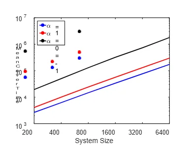
Figure 3.10: Mean cover time as a function of the system size, for power-law random walk exploration (with parameter𝛼) with various parameter values. The two axes are in log scale. Results are on Erd˝os-R´enyi graph with mean degree four. The straight-line behaviour we see implies a power-law dependence of mean cover time 𝜏 on the system size𝑁. It is of interest to know how much time it would take to cover the entire network with a 99 % success rate, as it could have potential applications, for instance, in the example of treasures mentioned earlier. In Fig. 3.9, we see the 1st and 99th percentiles of the distribution of cover times when unbiased network exploration is performed, as touched in the previous paragraph. We see that, with a 99 percent probability, the cover time is going to be less than 23117. So they only need to take 23117 steps to ensure they have covered the entire network with a 99 percent probability, in an average sense. Now we look at our analysis of the mean cover time⟨𝜏⟩, which is computed as⟨𝜏⟩= ∑︀𝑁�� number of simulations. Fig. 3.10 shows the variation in the mean cover time as a function of the system size for three diﬀerent exploration strategies – power-law exploration with parameter values of -1, 0 and 1, on a double logarithmic plot. We ﬁnd that the mean cover time is a power-law function of the system size –⟨𝜏⟩ 𝑁 indeed follows Eq. 3.21. Further, mean cover time⟨𝜏⟩ 𝑁 is a convex function of𝑁. For all the search strategies tried out we observed that𝛾>1. The power-law exponents obtained for the values of𝛼 considered are given in table 3.1. From Fig. 3.10, it can be noticed that the mean cover time decreases as𝛼is increased from -1 to 1, for the three values of𝛼tried out. As seen in Fig. 2.2 in chapter 2, the search eﬃciency 𝐵(𝛼) increases with an increase in𝛼up to a value of𝛼close to 1. So based on the information we see a negative correlation between the search eﬃciency and

Figure 3.11: Standard deviation𝜎 𝜏 (𝑁) as a function of the system size𝑁, for power-law random walk exploration (with parameter𝛼) with various parameter values. The two axes are in log scale. Results are on Erd˝os-R´enyi graph with mean degree four. The straight line behaviour we see implies that the mean cover time 𝜏 is a power-law function of the system size𝑁.

Table 3.1: The power-law exponents corresponding to the power-law behaviour (Eq. 3.21) of mean cover time 𝜏 as a function of system size𝑁, for a couple of values of the search parameter𝛼.

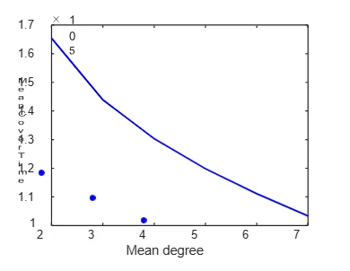
Figure 3.12: Mean cover time as a function of the mean degree for unbiased exploration on Erd˝os-R´enyi networks of size 3200. The Mean cover time decreases with increasing the mean degree, as the number of connections per node, and hence the number of paths available to the random walker per node increases. the mean cover time. That is something expected, as a more eﬃcient search strategy (one with larger𝐵) is likely to lead to a quicker exploration of the network (lesser mean cover time). In Fig. 3.11 we see the standard deviation𝜎 𝜏 (𝑁) as function of𝑁when power- law exploration is performed on Erd˝os-R´enyi networks of mean degree four. The double logarithmic plot shows that𝜎 𝜏 (𝑁) is a power-law function of𝑁(Eq. 3.22), and we ﬁnd that the power-law exponent (Eq. 3.22) is larger than 1. The power-law exponents computed for the three values of𝛼are as follows: . We compare power-law exponents𝛾 𝜏 for mean (Eq. 3.21) with power-law exponents𝜒for standard deviation (Eq. 3.22) and ﬁnd that𝛾 𝜏 >𝜒. The mean cover time as a function of the mean degree is shown in Fig. 3.12. If the mean degree of a graph is increased while keeping its size unchanged, there will be more connections per node, hence more paths available to explore. So one would expect to cover all nodes in a shorter time, which is what we see in Fig. 3.12. A close inspection of the plot (in log scale) reveals that the decay in⟨𝜏⟩with𝑐is faster than a power-law decay, based on the values of𝑐tried out. As a potential application of cover times, we can think of the example of treasures introduced earlier. It would of interest to know how many steps a person has to take to cover the given network 90 percent of the time in an average sense. To answer questions like that, we can refer to percentiles of the distribution of cover times. For the case of an exploration on an Erd˝os-R´enyi network of size 2000, the desired number is𝜏90 = 𝜇(2000) +𝜎 𝜏 (2000)𝑧90, as obtained from Eq. 3.25, in terms of normalised ﬂuctuations𝑧 90. Now, we turn to our results for the extreme value statistics of cover times. As a potential application, one could think of a real-world scenario where security forces are trying to ﬁnd a number of bombs hidden in some sites selected from a connected network of a large number of sites. Then the time it takes to cover all sites is an important quantity, as due to the nature of the threat posed by bombs, we cannot aﬀord to miss even one site. Also, the time it takes to cover all sites in extreme cases (𝜏takes the largest or smallest value over a set of random walks) is an important quantity too. With reference to that, in Fig. 3.13 we see the distribution of extreme values (maximum) of cover times for𝑠= 10 when unbiased explorations is performed on Erd˝os-R´enyi networks of size 200. In the left panel, we can see the 5th (leftmost vertical black line) and the 75th (rightmost vertical black line) percentiles, in addition to the mean value (middle black line). It is to be noted that we are showing the 75th percentile and not the 95th, which falls out of the range of the ﬁgure. Percentiles can have the signiﬁcance from a real-world perspective. In the right panel, one can see that the distribution of𝜏 𝑚𝑎𝑥 has a straight line behaviour in𝜏 𝑚𝑎𝑥, for large𝜏 𝑚𝑎𝑥.

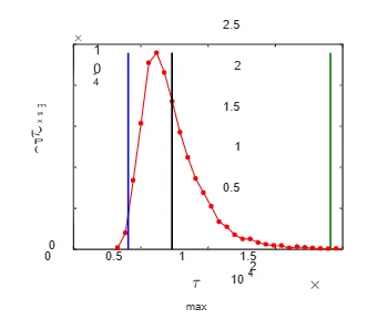
Figure 3.13: Distribution of the extremum (maximum) of cover times for𝑠= 10 when unbiased exploration is done on Erdos-Renyi network of size 200 and mean degree 4 (bin- width: 41). In the left panel, we see the normalised distribution (blue curve) and the 5st (leftmost black line) and 75th (rightmost black line) percentiles. The 1st percentile is 4073, and the 99th percentile is 19095. We also see the mean value of maxima of cover times (the middle black line), which is 7323. In the right panel, we see the probability density in the log scale. The straight line behaviour for large𝜏implies𝑃(𝜏 𝑚𝑎𝑥) decays exponentially (Eq. 3.20) for large𝜏 𝑚𝑎𝑥. The slope𝑏of the exponential ﬁt “ ln𝜏 𝑚𝑎𝑥 =𝑎−𝑏𝜏 𝑚𝑎𝑥” is

-0.0005±0.000015, and the intercept is 1.6±0.22

Figure 3.14: Normalised distribution of𝜏 𝑚𝑎𝑥 observed from the data obtained from sim- ulations (sim. in the plot) and the Weibull distribution ﬁt, for𝑠=10 and 16. Unbiased exploration performed on Erd˝os-R´enyi graphs of size 200 and mean degree four. It can be seen that the ﬁt is good.

Fig. 3.14 shows distributions of maximum of cover time for two diﬀerent values of𝑠 number of random walks over which maximum is taken. We also see the corresponding Weibull distributionﬁt. As one can see, based on the ﬁt, it can be concluded that the distribution of extremum of cover times belongs to the Weibull extreme value class. In the next part, we present a summary of the chapter.

3.6 Summary & Discussion

In this chapter, we carry out a numerical analysis of the ﬂuctuations and extreme value statistics of random walk exploration and search on complex networks. Speciﬁcally, the focus has been on mainly two quantities arising from random walk exploration – cover times and𝑆(𝑛),which is a measure of network exploration eﬃciency. We have also investigated random walk search based quantity𝑆(𝜉,𝑛) – the number of items found in 𝑛time steps. Our analysis concerns Erd˝os-R´enyi graphs. The two tools, namely, the cavity method and the population dynamics approach, used for the computation of the average search eﬃciency and the average exploration eﬃciency in Chap. 2 cannot help with understanding the nature of the ﬂuctuations of the exploration eﬃciency and the search eﬃciency. In this chapter, to understand the ﬂuctuations of those quantities, we go beyond the tools used in the previous chapter and take a numerical simulations route to understand theﬂuctuations. The numerical analysis of the ﬂuctuations of exploration eﬃciency (measured as𝑆(𝑛)) reveals that the distribution of the normalised ﬂuctuations is independent of𝑛and𝑁, as long as𝑛≫1. It is, however, dependent on the graph type, mean degree, and exploration strategy. We further ﬁnd that the distribution of each of the network exploration eﬃciency and the search eﬃciency is non-symmetric about its mean. We looked at the behaviour of the standard deviation𝜎(𝑛) of𝑆(𝑛) as a function of𝑛. It is found that𝜎(𝑛) is a power-law function of𝑛, with the power-law exponent being a value close to 1/2. Since the degree-biased random walks under consideration, particularly on large networks, have an eﬀective drift, these random walks resembles one-dimensional random walks with a drift, for which, it is known that the standard deviation over a 1 𝑛-step walk is proportional to𝑛 2 . Given the resemblance, the true power-law exponent in our case may be 1/2.

We investigate the extreme value statistics of𝑆(𝑛), where the extremum of𝑆(𝑛) is taken over a set of independent random walks. We ﬁnd that the distribution of extreme values of𝑆(𝑛) is Weibull – one of the three standard classes of the Generalised Extreme Value distributions – in nature, which is something expected given the boundedness of 𝑆(𝑛). We also analyse the dependence of the location parameter of the Weibull distribution ﬁt on the number of sets of random walks over which maximum/minimum is taken, and weﬁnd that the dependence is sub-power-law. Now we turn to cover times. Studying the probability distribution of the cover time 𝜏, we conﬁrmed that, for large𝜏, the probability𝑃(𝜏) of having the cover time in range [𝜏,𝜏+ d𝜏) has an exponential decay with𝜏. This was one of the results of analytical study [33] on cover times by Chupeau et al., and we conﬁrm the result from a numerical simulations approach. We have also analysed the dependence of the mean cover time⟨𝜏⟩ 𝑁 and the standard deviation of cover times𝜎 𝜏 (𝑁) on the system size𝑁, and weﬁnd that both the quantities have a power-law dependence on the system size. The power-law exponents for both the power-law behaviours were found to be larger than 1 for a family of degree-biased exploration strategy. The analysis of the eﬀect of the exploration strategy (speciﬁcally, the search parameter 𝛼for power-law search strategy) on the cover time and the exploration eﬃciency reveals that there is a negative correlation between the mean cover time and search eﬃciency𝐵, which was computed in chapter 2. In other words, a more eﬃcient search strategy leads to a smaller mean cover time, which is something one would expect. We now come to the extremum of cover times, taken over a set of random walk explorations. We notice that the degree distribution of the maximum of the cover time, 𝜏𝑚𝑎𝑥, has an exponential shape for large𝜏. We ﬁnd that the distribution of𝜏 𝑚𝑎𝑥 belongs to the Weibull extreme value class, even though the cover times are unbounded. In the next chapter, we present our inferences from the learning for the hider and seeker in the game of hide-and-seek. That includes: 1) learning from his performance so far in the same game, for the seeker and 2) learning from the performance in the previous games for the two players when repeated games are played.

Chapter 4 Learning in Hide-and-Seek Games

Introduction

There are many scenarios in real-life involving searching for something by a party. For example, a police oﬃcer is searching for a thief hidden in some room in a big hotel. Another example is of a person searching for hidden treasures in a group of sites. Such scenarios as we know from before can be formalised as a search game for the purpose of modeling them. Search games have potential applications in a variety ofﬁelds [47]. Applications of search games in theﬁeld of economics are discussed by Aumann et al. [52]. A recent comprehensive survey [53] of search games provided by Hohzaki covers many applications of search games. Search games have many times and can be studied from various contexts. For instance, Kikuta study a two-person zero-sum hide-and-seek game [54] on a straight line from a game theory perspective, where they try toﬁnd the equilibrium strategies for the two players playing the game using concepts such as mathematical induction. On the other hand, Chapman et al. [55] study a two-player hide-and-seek game on networks from a random walk perspective, where they investigate stochastic random walk simulations to pick the best strategy from a pool of random walk strategies. We in this work, including in this chapter, take a random walk simulations approach to study hide-and-seek games on complex networks.

Methodology

Now we turn to the methodology for this study of learning in the game of hide-and- seek. Here we investigate learning for both the players individually from their past search performance when repeated rounds of games are played on Erd˝os-R´enyi graphs. The goal of learning for the players is optimisation. The seeker is looking to maximise the search performance whereas the hider is looking to minimise the search performance. Let us revisit how the game of hide-and-seek is played. First the hider picks a set of nodes on the network based on a hiding strategy and a given percentage occupancy and hides one item each on these nodes. Then the seeker starts at a node picked at random and performs a random walk as per a search strategy. The seeker keeps moving until all the hidden items are found, and that’s when the game is over. In this study the search strategy under consideration is the degree-biased random walk search (Eq. 2.7) and the hiding strategy (Eq. 2.20) under consideration is the degree- biased random hiding. To be more speciﬁc, we experiment with degree-biased power-law random walk strategy for search and degree-biased power-law strategy for hiding, both of which are given in table 2.1. In the learning process, repeated rounds of multiple games are played. All games in each round correspond to the same search and hiding strategies. In case of learning for the seeker individually, after each round the search strategy is updated based mostly on the outcome of the last update in the search strategy, sometimes on the collective outcome of last few updates. By outcome we mean the change in the search eﬃciency, or the search performance, which is measured by the average number of items found in𝑛time steps over a set of𝑛-step random walks. In case of learning for just the hider Continuing from above, the goal with regard to learning for the seeker is strategy optimisation, or parameter optmisation if a family of search strategy is picked. In each game in a round,𝛼has the same value. After each round,𝛼is amended based on whether the most recent update in𝛼has led to a higher search eﬃciency or not. If it has led to higher search eﬃciency, then the next update is going to be in line with the last update, i.e., if last update was𝛼→𝛼+ d𝛼, then the next update is also going to be𝛼→𝛼+ d𝛼. If it has led to a lower eﬃciency, then the current update is going to be𝛼→𝛼−d𝛼/2. We either stop updating𝛼when the change in the search eﬃciency with respect to a change in𝛼is within the error zone of 𝑆¯(𝜉,𝑛), or have a number of random walk rounds further that could be used to compute a more robust 𝑆¯(𝜉,𝑛), and hence the search eﬃciency𝐵. The learning routine for exploration and hiding can be described likewise.

Chapter 5 Summary

In this thesis, we investigate random walk strategies for search and exploration on complex networks. There are two main parts of this work. In theﬁrst part, we compute the average search and exploration eﬃciencies, investigate the search performance for families of degree-biased random hiding and degree-biased random walk searching strategies, and present two approximations to the average exploration eﬃciency. In the second part, we numerically investigate theﬂuctuations in the exploration and search eﬃciency, in addition to investigating the extreme value statistics of random walk exploration eﬃciency. In theﬁrst part of this thesis, to start with, we extend De Bacco et al.’s result [76] of the average exploration eﬃciency for unbiased random walk exploration on complex networks to the case of degree-biased random walk exploration. Further, we bring in the aspect of hiding as per the hide-and-seek games on complex networks and compute the average search eﬃciency corresponding to a set of hidden items. We verify that the average search and exploration eﬃciencies obtained from random walk simulations performed are in excellent agreement with those obtained from the cavity method. Going a step further from the computation of the average exploration eﬃciency using the cavity method, we compute the average exploration eﬃciency in the thermodynamic limit, on the giant component of the graph, using tools from Ku¨hn’s work on disentangling the giant component [98]. Our thermodynamic limit results are in excellent agreement with those obtained from the cavity method and random walk simulations. It can further be noticed from the expression of average exploration eﬃciency that it can be written as a sum of𝑘-speciﬁc contributions from nodes of degree𝑘, and we formally write the expression for those𝑘-contributions for degree𝑘nodes.

As the computation of the average exploration and search eﬃciencies can be computa- tionally expensive at times, we introduce two approximations to it. Theﬁrst one based on the idea that the distance between the equilibrium distribution of searcher’s position on the network and the distribution of hidden items is likely to be small for eﬃcient search strategies. The second one is based on the assumption that any step of a non-backtracking random walk would explore parts of the network not seen before, and the approximation is expected to be good on networks with typically large degrees. We show that the second approximation is good even on Erd˝os-R´enyi graphs with modest mean degrees. We study the hide-and-seek interplay for parameterised families of random walk searching and random hiding strategies, with the aim to do search eﬃciency maximisation for the searcher, and search eﬃciency minimisation for the hider. It is found in all cases tried out that, for a given family of degree-biased hiding strategy, the most search eﬃcient member of the same family of degree-biased search strategy performs better than the most search eﬃcient member of a diﬀerent family of degree-biased search strategy. When parameterised searching is carried out, for a given hiding strategy, it is generally found that an intermediate value of the search parameter results in the optimisation of the search eﬃciency, and a similar statement can be made for the exploration eﬃciency, on a network with a non-uniform degree distribution. Very large or small values of the search parameter generally result in a low search eﬃciency. The reason for that is, extreme values of the parameter would generally make the searcher spend quite a bit of time on either a set of low degree nodes or a set of high degree nodes, hence hindering the process of uncovering of new sites at a fast pace. We found that, for a given hiding and searching strategies, the search eﬃciency𝐵(𝜌 ℎ) for percentage occupancy𝜌 ℎ is proportional to𝜌 ℎ. Further, for a given hiding strategy, the normalised search eﬃciency𝐵(𝜌 ℎ)/𝜌 ℎ can be larger than 1 for certain search strategies, a result that can be exploited well when deciding which search strategy to go for.

When comparing graph types, we ﬁnd that, for degree-biased search with intermediate values of the search parameter so that the bias towards high or low degree nodes is not too small or too large, a higher search eﬃciency is obtained on scale-free graphs than on Erd˝os-R´enyi graphs. That is because of the presence of relatively large degree hubs in scale-free graphs, which implies more connecting nodes, and hence more paths available to explore. For extreme values of the search parameter, the eﬃciency on both the graph types is small due to localisation issues. On random regular graphs, the search eﬃciency is constant with any change in the value of the search parameter, as there is no topological bias. The focus so far, in the ﬁrst part of the thesis (Chap. 2), has been on determining the average search and exploration eﬃciencies. In the second part of this thesis (Chap. 3), we moved to investigate the ﬂuctuations and extreme value statistics of search and exploration eﬃciencies. As ﬂuctuations and extreme values are out of reach of the analytical tools used in Chap. 2, we used numerical simulations instead in Chap. 3. The numerical analysis of the ﬂuctuations of the exploration eﬃciency reveals that the distribution of these normalised ﬂuctuations (normalised ﬂuctuations of𝑆(𝑛), to be precise, which is a measure of the exploration eﬃciency) is independent of𝑛and𝑁, as long as𝑛≫1. But it is dependent on the graph topology, including the graph type and the mean degree, and the exploration strategy. Further, each of the distributions of the network exploration and search eﬃciencies is found to be non-symmetric about its mean, and the degree of non-symmetry is inﬂuenced by the search strategy, among possibly other factors. Due to the eﬀective drift of random walks on graphs with typically large degrees, the random walk on such graphs closely resemble one-dimensional random walk with a drift, 1 Where, the standard deviation after𝑛steps is proportional to𝑛 2 . In view of this close resemblance, it seems that the exponent of the power-law dependence of𝜎(𝑛) in𝑛might also be 1/2. Our analysis of the ﬂuctuations of maximum or minimum of𝑆(𝑛), where each maxi- mum or minimum is taken over a set of independent random walk explorations of𝑛step each, reveals that the probability distribution of the maximum or minimum of𝑆(𝑛) be- longs to the Weibull Extreme Value distributions family. It is an expected result given the boundedness of𝑆(𝑛), where it is bounded above by𝑛, and bounded below by 1 for 𝑛= 1, and 2 for𝑛>= 2. Turning to cover times, we investigate the distribution of cover times, analyse the behaviour of the mean and variance of cover times as a function of the system size, and study the extreme value statistics of cover times, all on Erd˝os-R´enyi graphs. We ﬁrst conﬁrm Chupeau et al.’s result from their analytical study [33] on Erd˝os-R´enyi networks that, for large𝜏, the probability𝑃(𝜏) of having the cover time in the range [𝜏,𝜏+ d𝜏) has an exponential decay with𝜏.

Continue your journey with our comprehensive guide to Boosting Motivation through Gender Groups .

Weﬁnd that, on Erd˝os-R´enyi graphs, the mean cover time⟨𝜏⟩ 𝑁 on systems of size𝑁, when viewed as a function of𝑁, has a power-law dependence on𝑁. The same can be said for the standard deviation𝜎 𝑁 (𝜏) of cover times on systems of size𝑁. Further, the power-law exponents for both the power-law dependencies are more than one. The power- law exponent for mean cover time dependence is typically larger than the corresponding value for the standard deviation𝜎 𝑁 (𝜏). For degree-biased power-law random walk exploration strategy, weﬁnd that the mean cover time is negatively correlated with search eﬃciency𝐵computed in chapter 2. In other words, a more eﬃcient exploration strategy, which implies a larger𝐵, leads to a smaller cover time, and vice-versa, which is something one would expect. Coming to the distribution of the maximum of the cover time over many independent random walk explorations,𝜏 max, we ﬁnd that distribution of𝜏 max belongs to the Weibull extreme value class. And the same can be said about the distribution of the minimum of the cover time. Further, the distribution of𝜏 max is exponential in shape for large𝜏 max.

A paragraph or two on learning!

Our investigation of random walk exploration and search eﬃciencies in this thesis has been restricted to degree-biased random walk strategies. A wider class of random walk search strategies can be tried out. Examples include the random walk with restart (RWR). In a RWR, at any step, the walker makes a transition, with probability𝑟(0 𝑟 1), to one of its neighbours, or hops to the starting node (in case of single starting node) with probability 1−𝑟. Also, intermittent random walks can be a good candidate for the search strategy. During an intermittent random walk, at any step, the walker can go to one of its neighbours with probability𝛼, lying between 0 and 1, and jump oﬀ-network with probability 1−𝛼. Our analysis of the hide-and-seek interplay in this thesis was restricted to the case where, at each site, there is either one item or there is no item. This criterion can be relaxed and search eﬃciencies could be investigated for a variety of distributions of the number of hidden items across the network.

What Makes Us Unique

24/7 Customer Support
100% Customer Satisfaction
No Privacy Violation
Quick Services
Subject Experts

Optimizing Search in Complex Networks

Chapter 1 Introduction

Chapter 3 Random Walk Exploration and Search on Complex Networks: Fluctuations and Extreme Values

Introduction

Average Exploration Eﬃciency

Exploration Eﬃciency

Fluctuations of Exploration Eﬃciency

Extreme Values of Exploration Eﬃciency

3.3.2.1 Extreme Values: Formulation and Distribution

3.3.2.2 Generalised Extreme Value Distributions

Cover Time Analysis

Distribution of Cover Times

Normalised Fluctuations and Extreme Values

3.5 Results

3.5.1 Fluctuations of Network Exploration and Search Eﬃcien- cies

3.5.2 Extreme Value Statistics of Network Exploration Eﬃciency

3.5.3 Cover Time Analysis

3.6 Summary & Discussion

Chapter 4 Learning in Hide-and-Seek Games

Introduction

Methodology

Chapter 5 Summary

Place Your Assignment Request

What Makes Us Unique

Dissertation Samples

Assignment/Essay Samples

Research Proposal Samples